Deep Learning Explained: How Neural Networks Actually Work

Deep learning is responsible for most of the AI capabilities that feel genuinely impressive right now — image recognition that outperforms human radiologists, language models that write code, voice assistants that understand Tamil spoken in a Chennai accent, self-driving vehicles navigating complex traffic. Understanding how it actually works — not just that it works, but the mechanism — gives you a foundation for learning any specific deep learning application, debugging models when they fail, and making informed decisions about when to use it and when not to.

This guide explains deep learning from the ground up. No shortcuts that sacrifice accuracy, but also no unnecessary mathematical formalism. By the end, you should understand what a neural network is, how it learns, what makes deep networks powerful, and what their genuine limitations are.

What a Neural Network Actually Is

A neural network is a mathematical function. It takes inputs, applies a sequence of transformations to them, and produces outputs. That is all it is. The "neural" framing is a metaphor drawn from a loose analogy to biological neurons, but the analogy is imprecise enough that it can mislead. Focus on the mathematics.

The basic building block is a neuron (or node), which computes:

output = activation_function(weights · inputs + bias)

Where:

• inputs is a vector of values coming into this neuron
• weights is a vector of learned parameters controlling how much each input matters
• bias is a single learned parameter that shifts the output
• activation_function introduces non-linearity (more on this in a moment)
• · denotes the dot product — multiply each weight by its corresponding input, sum the results

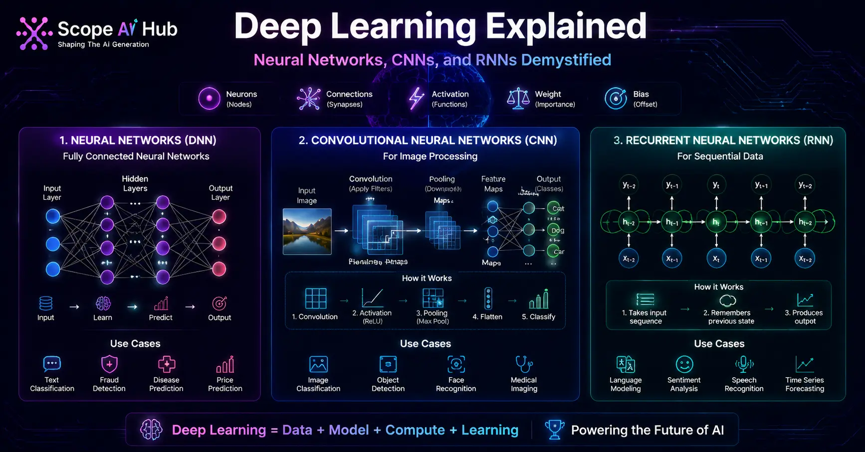
Neurons are organized into layers. All neurons in the same layer receive the same inputs (from the previous layer) and their outputs all feed into the next layer. A network with multiple layers between input and output is called "deep" — this is where "deep learning" comes from.

Why Depth Matters: Hierarchical Feature Learning

The key insight behind deep learning is that stacking layers allows a network to learn hierarchical representations — features built on top of features.

Consider how a deep network learns to recognize faces in images. The first layer might learn to detect edges — horizontal lines, vertical lines, diagonal lines, at various positions. The second layer combines edge detectors to form detectors for curves, corners, and simple shapes — eyes as circles, noses as triangles. The third layer combines these into part detectors — an eye-like pattern, a nose-like pattern. Deeper layers combine parts into full face representations.

No human engineered these intermediate representations. The network learned them automatically from labeled examples. This is the remarkable property of deep learning: given enough data and compute, it discovers useful intermediate representations on its own.

This is why deep learning dramatically outperformed earlier AI methods on problems involving images, audio, and text — domains where hand-engineering good features was prohibitively difficult or impossible.

The Non-Linearity Requirement

If each neuron only computed a weighted sum (no activation function), then no matter how many layers you stacked, the entire network would still be equivalent to a single linear function. Stacking linear functions produces another linear function.

Non-linear activation functions break this — they allow the network to represent curved decision boundaries and complex relationships. The most commonly used activation today is ReLU (Rectified Linear Unit):

ReLU(x) = max(0, x)

Simple but effective. It outputs 0 for negative inputs and the input value unchanged for positive inputs. Its simplicity makes it computationally fast and avoids the vanishing gradient problem that plagued earlier activation functions (sigmoid, tanh) in deep networks.

How Networks Learn: Gradient Descent and Backpropagation

A neural network starts with random weights. Through training, it adjusts those weights to minimize its errors on the training data. This process has two parts.

The Loss Function

First, you need to measure how wrong the network's predictions are. The loss function (or cost function) computes a number representing the total error across a batch of training examples.

For regression (predicting continuous values): Mean Squared Error (MSE) — average squared difference between predictions and true values. Large errors are penalized more than small ones.

For classification (predicting categories): Cross-Entropy Loss — measures how far the predicted probability distribution is from the true one-hot distribution. A confident wrong prediction gets a much higher loss than an uncertain wrong prediction.

Gradient Descent

The network minimizes the loss by adjusting its weights in the direction that decreases the loss most rapidly. This direction is the negative gradient of the loss with respect to each weight — for each weight parameter, how does a small change in that weight affect the loss?

The update rule:

weight = weight - learning_rate × gradient

The learning rate controls how large each step is. Too large: the updates overshoot the minimum and the loss oscillates or diverges. Too small: training is extremely slow. Finding a good learning rate is one of the most important hyperparameter choices in practice.

Modern optimizers (Adam, AdamW) adapt the learning rate automatically per parameter, which makes training more robust than fixed learning rates.

Backpropagation

Computing the gradient of the loss with respect to every weight in a network with millions of parameters requires an efficient algorithm. Backpropagation applies the chain rule of calculus to propagate error gradients backward through the network — from the output layer toward the input layer.

The chain rule says: if y depends on x through z (y = f(z), z = g(x)), then dy/dx = dy/dz × dz/dx. Backpropagation applies this recursively across all layers, computing each layer's weight gradients from the gradient passed back from the layer above it.

Deep learning frameworks (PyTorch, TensorFlow) implement automatic differentiation — they track all mathematical operations performed in the forward pass and automatically compute gradients in the backward pass. You define the forward computation; the framework handles backpropagation automatically.

Core Architectures

Different problem types call for different network architectures. The architecture specifies how neurons are connected and what kinds of transformations they apply.

Feedforward Networks (Fully Connected / MLP)

The basic architecture: each neuron in one layer connects to every neuron in the next layer. Suitable for tabular data where the spatial or sequential structure of the input does not matter. Used for simple classification and regression on structured features.

Convolutional Neural Networks (CNNs)

Designed for spatially-structured data, particularly images. Instead of connecting every input pixel to every neuron (which would require enormous numbers of parameters), convolutional layers apply learned filters that slide across the image, detecting local patterns regardless of where they appear.

A 3×3 filter for edge detection looks for the same pattern at position (10, 10) and position (200, 200) — the same filter is shared across the entire image. This parameter sharing dramatically reduces the number of learned weights and builds in translational invariance (a cat in the top-left corner and a cat in the bottom-right corner are both recognized as cats).

CNNs dominate image classification, object detection, medical imaging, and video analysis.

Recurrent Neural Networks (RNNs) and LSTMs

Designed for sequential data — text, speech, time series — where the order of inputs matters. RNNs maintain a hidden state that is updated at each time step, allowing the network to carry information forward through a sequence.

Long Short-Term Memory (LSTM) networks introduced gating mechanisms that allow the network to selectively remember and forget information, which dramatically improved performance on long sequences where basic RNNs struggled with vanishing gradients.

LSTMs dominated NLP and speech recognition from roughly 2014 to 2018 before being largely displaced by transformers.

Transformers

The architecture behind every large language model (GPT, Claude, LLaMA, BERT), the best image models (ViT, DALL-E), and the most capable multimodal systems.

Transformers process input sequences using self-attention: for every element in the sequence, the network learns which other elements are most relevant and how much to weight their influence. Unlike RNNs, this is computed in parallel across the entire sequence, which makes transformers dramatically faster to train on modern GPU hardware.

The attention mechanism is also why transformers handle long-range dependencies so well — the relationship between a word at position 1 and a word at position 500 is computed with the same computational cost as two adjacent words.

What Deep Learning Cannot Do

Understanding the limitations is as important as understanding the capabilities.

Data hunger. Deep networks require large amounts of labeled training data to generalize well. The ImageNet dataset that enabled the 2012 deep learning breakthrough had 1.2 million labeled images. Building labeled datasets at scale is expensive and time-consuming, and for specialized domains (medical imaging, rare defect types) the required data may not exist.

Interpretability. A logistic regression model's predictions can be explained by examining its coefficients. A 70-billion parameter transformer's predictions cannot be explained in any similarly intuitive way. This matters enormously in regulated industries — banking, healthcare, insurance — where models must be auditable.

Out-of-distribution generalization. Deep learning models learn patterns from their training distribution. When they encounter inputs that look different from training data in ways that would not confuse a human, they can fail in unexpected and overconfident ways. An image classifier trained on well-lit Indian urban traffic may fail on rural night conditions even though both are "traffic images."

Causality. Deep models learn correlations, not causal relationships. A churn prediction model might learn that customers who contact support twice within a month are at high risk of churning. But does the support contact cause churn, or are both symptoms of the same underlying problem? The model cannot tell you. Intervening to reduce support contacts (instead of fixing the root problem) might make things worse.

The Path Into Deep Learning

Understanding deep learning conceptually is the starting point. Being able to build and deploy deep learning systems — writing PyTorch training loops, fine-tuning pretrained models, debugging training runs, deploying to production — is what employers pay for.

Our Machine Learning and Deep Learning course moves from these conceptual foundations through hands-on implementation in PyTorch, covering feedforward networks, CNNs for image tasks, and transformer-based NLP. The prerequisite is comfort with Python and basic statistics — our Python for AI and Machine Learning course covers the required foundation.

Frequently Asked Questions

Q: How is deep learning different from machine learning? A: Deep learning is a subset of machine learning. Machine learning is the broad approach of learning from data. Deep learning specifically refers to using neural networks with many layers (deep networks). Not all machine learning is deep learning — gradient boosting, random forests, and SVMs are machine learning methods that are not deep learning.

Q: Do I need a GPU to learn deep learning? A: Not to start. Google Colab provides free GPU access that is sufficient for learning and smaller projects. Once you are training larger models or working with significant amounts of data, your own GPU or cloud compute becomes necessary. For the learning phase, Colab is sufficient.

Q: Is deep learning always the best approach? A: No. For tabular business data (the most common type in Indian enterprise applications), gradient boosting (XGBoost, LightGBM) typically matches or outperforms deep learning with less data and less tuning effort. Deep learning's advantages are most clear for unstructured data — images, text, audio — and for very large datasets.

Q: How long does it take to learn deep learning? A: Enough to build and train basic networks: 2-3 months with consistent practice. Enough to contribute meaningfully to a production deep learning project: 6-12 months. Enough to push the research frontier: years. Focus on being productive at the middle level first — that is what most industry roles require.

---

Ready to Go from Theory to Building Real Neural Networks?

Our Chennai batches cover deep learning end to end — architecture understanding through PyTorch implementation and deployment.

📞 Call/WhatsApp: +91 70102 30379 📧 Email: info@scopeaihub.com 📍 Visit Us: 10, Tilak St, T. Nagar, Chennai – 600017 🌐 Website: www.scopeaihub.com